What Is LLM Inference, Really? A Deep Technical Walkthrough

Let me be honest with you. When I started working on LLM infrastructure, I had eleven years of distributed systems experience. I knew Kafka, Kubernetes, Prometheus. I could debug a partition rebalance in my sleep.

And yet the first time someone asked me what actually happens during inference, I said something like “the model reads the prompt and generates tokens.” Which is technically true the same way “a database reads your query and returns rows” is technically true — accurate, useless, and deeply embarrassing for someone drawing a principal engineer’s salary.

This post is what I wish I’d had on day one. We’re going to walk through the entire inference pipeline — from the moment your request arrives to the moment you see text on screen — with real examples, honest explanations of where the performance goes, and enough detail that you can actually reason about production problems.

No “and then the transformer does its thing.” No skipped steps. Strap in.

1. What Is Inference?

Training is where you take a massive dataset, run it through a model millions of times, and slowly adjust billions of numerical weights until the model gets good at predicting the next word. Training is done once (or occasionally). It costs millions of dollars in GPU-hours and requires a team of researchers.

Inference is what happens afterward, every time someone uses the model. It’s the model using those learned weights to respond to new input. No weights change. No learning happens. It’s pure forward-pass computation.

Think of it like this: training is baking the bread. Inference is slicing it and serving it to customers. The bread (weights) is done. The kitchen (inference engine) just has to plate it fast enough that the queue doesn’t back up to the street.

The inference engine is the runtime that takes the frozen model weights and executes them against an input. The same weights can run on Ollama, vLLM, TensorRT-LLM, or TGI — and get meaningfully different performance from each. The weights don’t change. The execution strategy does.

This distinction matters operationally: inference is not a solved problem. Serving a model efficiently at scale is a full engineering discipline.

2. The Artifact: What’s Actually in That 10GB Download?

When you run ollama pull mistral or grab a model from HuggingFace, you aren’t just downloading a “program.” You’re downloading a massive, frozen brain in a box. If you’ve ever wondered why a model that “just chats” takes up 10GB of your SSD, it’s because it is packed with billions of tiny numerical “preferences” the model learned during its training phase.

Think of the GGUF (or Safetensors) file as a giant Ikea flat-pack box. To build the working model, you need two things: the Instruction Manual and the Hardware.

What’s inside a 7B parameter model file:

GGUF file structure (simplified):
├── Header
│   ├── Model architecture (LlamaForCausalLM)
│   ├── Vocabulary (32000 tokens + their embeddings)
│   ├── Context length (4096, 8192, etc.)
│   └── Hyperparameters (n_layers, n_heads, etc.)
│
└── Weight tensors:
    ├── token_embeddings        [32000 × 4096]   ← the embedding matrix
    ├── layer.0.attention.q     [4096 × 4096]    ← Query projection weights
    ├── layer.0.attention.k     [4096 × 4096]    ← Key projection weights
    ├── layer.0.attention.v     [4096 × 4096]    ← Value projection weights
    ├── layer.0.attention.out   [4096 × 4096]    ← Output projection
    ├── layer.0.ffn.up          [4096 × 11008]   ← Feed-forward up
    ├── layer.0.ffn.down        [11008 × 4096]   ← Feed-forward down
    ├── ... × 32 layers
    └── output_norm + lm_head   [32000 × 4096]   ← Final projection to logits

The “Manual” (The Header)

This is the first few kilobytes of the file. It tells the inference engine (like Ollama or vLLM) how to put the brain together. It includes:

The Architecture: Identifies the model type (e.g., LlamaForCausalLM) so the engine knows which math rules to apply.
The Vocabulary: A dictionary of roughly 32,000 to 128,000 “tokens” (the syllables the model speaks).
The Hyperparameters: Crucial settings like the number of layers (32 or 80) and the context length (how much it can remember).

The “Hardware” (The Tensors)

The rest of that file is just rows and rows of numbers called Weights. Every inference request is essentially looking up values from these matrices and multiplying them together—32 times over.

The “Part”	What it actually does in plain English
`token_embeddings`	The Translator. Turns human text into the model’s internal number-language.
`attention.q, k, v`	The Highlighters. Helps the model decide which part of your sentence is important.
`ffn.up` & `ffn.down`	The Reasoning Muscles. Does the heavy lifting of processing and transforming information.
`lm_head`	The Microphone. Turns the final internal math back into a word you can read.

Quantization: Shrinking the Brain

You might notice some files are 15GB while others are 4GB for the same model. This is Quantization—the art of compression. We turn high-precision 16-bit floats into lower-precision integers (like 4-bit).

Precision	Bits per weight	7B Model Size	The SRE Reality
FP16	16	~14GB	Requires an A100. Pristine quality.
INT8	8	~7GB	Fits on a high-end gaming GPU. Minimal loss.
INT4 (Q4_K_M)	4	~4GB	The Sweet Spot. Fits on a MacBook. Faster throughput.

Why SREs love INT4: Lower precision = smaller tensors = faster memory transfers. Because decoding is memory-bound, an INT4 model often delivers 20-40% better TPOT (tokens per second) than the “full” version because the memory bus isn’t screaming as loud.

The takeaway: You aren’t executing code; you are loading a massive, math-heavy lookup table. GGUF is your single-file “box,” and quantization is how you fit that box into a smaller truck (your GPU).

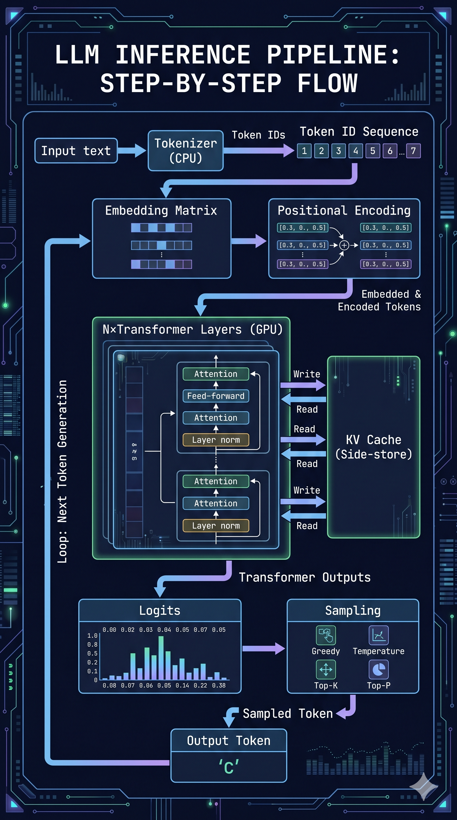
3. The Three Phases: A Map Before the Territory

Every inference request goes through three broad phases. They are not equally expensive, not equally parallelizable, and not equally friendly to your p99 latency.

┌──────────────────────────────────────────────────────────────────┐
│  TOKENIZATION  │  Prefill (Prompt Processing)   │ Decode         │
│    (CPU)       │           (GPU, compute)       │ Loop(GPU, Mem) │
│                │                                │                │
│                │                                │ current →      │
│  Text → IDs    │  Embed → Position → Attention  │ next token     │
└──────────────────────────────────────────────────────────────────┘
     Fast          Scales with prompt length        Slow

Tokenization: Split the text into token IDs the model understands. CPU-bound. Fast.
Prefill: Process the entire prompt through the model. GPU compute-bound. Scales with prompt length.
Decode: Generate output tokens one at a time. GPU memory-bound. Runs in a loop until done.

Each phase has its own bottleneck. Let’s go through them one by one.

4. Tokenization: Chopping Text Into Numbers

Before a single GPU operation happens, your text has to be converted into a format the model can work with: a sequence of integers called token IDs.

A token is not a character, and it’s not a word. It’s a chunk of text that appears frequently enough in the training corpus to deserve its own ID. There are several ways to build this vocabulary — WordPiece (used by BERT), Unigram (used by SentencePiece), and others — but the dominant approach in modern LLMs is Byte Pair Encoding (BPE): a compression algorithm that iteratively merges the most common pairs of characters or subwords into single tokens until it reaches a target vocabulary size.

The result is a vocabulary of roughly 32,000–128,000 tokens, each with a corresponding integer ID. The model never sees your text — it sees a list of numbers.

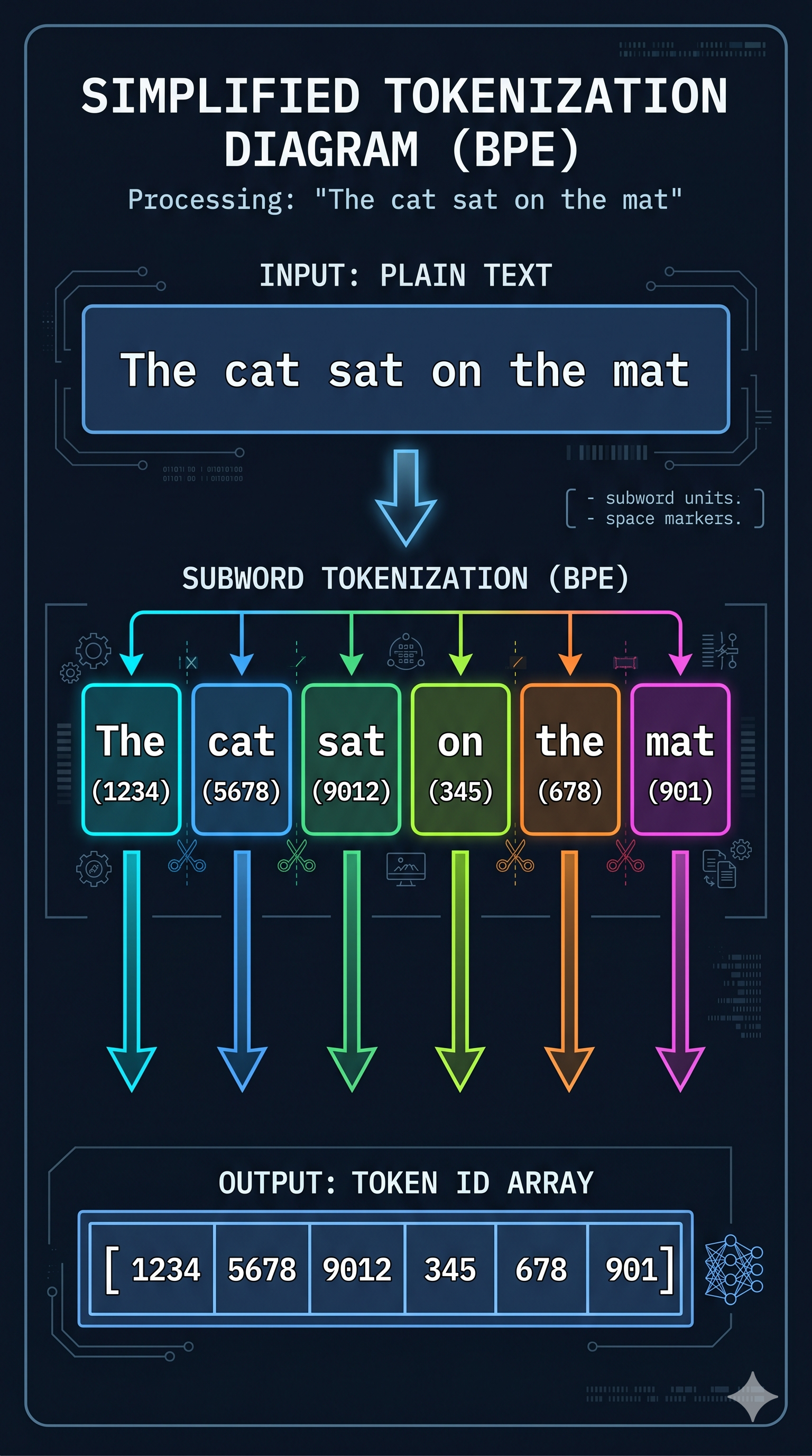
Take our example prompt: "The cat sat"

After tokenization, this becomes something like:

"The"  → 1026
" cat" → 5992
" sat" → 3290

Token IDs: [1026, 5992, 3290]

Note the space before “cat” and “sat” — it’s part of the token. Tokenizers care about whitespace because it affects meaning and frequency.

Is Tokenization CPU-Bound?

Yes. The tokenizer is usually written in Rust (HuggingFace’s tokenizers crate) or C++ for exactly this reason. For most requests it’s fast enough to be invisible — microseconds for a short prompt.

Where it bites you: very long documents fed to batch processing jobs. A 100,000-token context requires processing 100,000 token lookups. It’s still fast relative to GPU work, but it’s the one step in the pipeline running on CPU that you can’t just throw more GPU at.

How it’s improved: Parallelizing tokenization across CPU cores for batch workloads. Or — and this is the real fix — not re-tokenizing the same content repeatedly. If you have a shared system prompt you send to every request, tokenizing it once and caching the result is free latency.

5. Prefill: The Model Reads Your Prompt

Now we have token IDs. The model needs to turn those IDs into something it can reason about. This is prefill — the model processing the entire prompt in one shot.

Prefill has two sub-steps that are easy to conflate: embedding lookup and the actual transformer forward pass. Let’s take them in order.

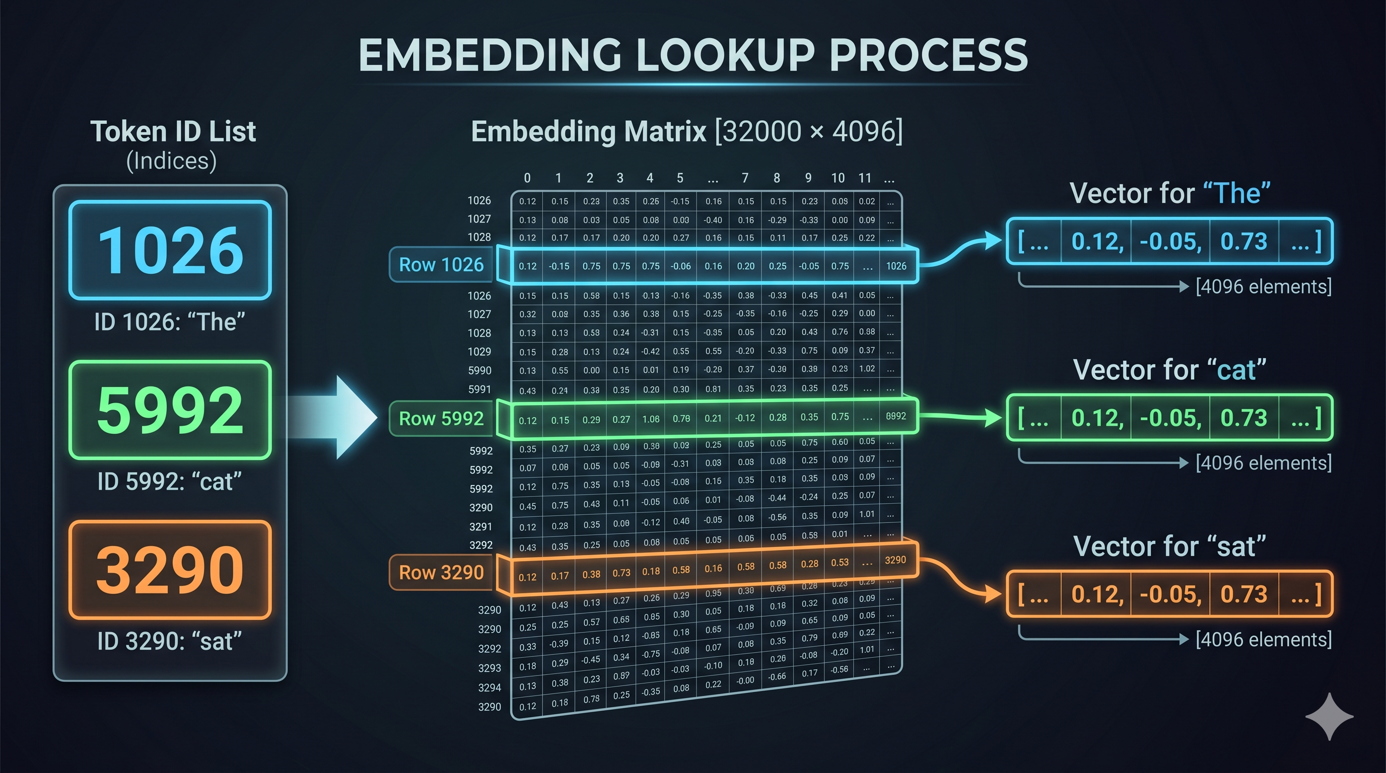
The Embedding Matrix

Every token ID maps to a high-dimensional vector of floating-point numbers called an embedding. These vectors live in the model’s embedding matrix — a giant lookup table with one row per vocabulary token and one column per embedding dimension.

For a model with a 32,000-token vocabulary and 4,096 embedding dimensions, this matrix has shape [32000, 4096]. At 16-bit float precision, that’s about 256MB just for the embedding layer.

Our example [1026, 5992, 3290] becomes:

Token ID 1026 → embedding row 1026 → [0.12, -0.43, 0.81, ..., 0.07]  (4096 values)
Token ID 5992 → embedding row 5992 → [-0.34, 0.91, 0.12, ..., -0.22] (4096 values)
Token ID 3290 → embedding row 3290 → [0.67, 0.05, -0.88, ..., 0.44]  (4096 values)

I’m simplifying to 8 dimensions here so this fits on a page. In reality it’s 4,096 or 8,192 dimensions depending on the model.

Simplified (3D instead of 4096D), just to show the shape:

"The"  → [0.12, -0.43,  0.81]
" cat" → [-0.34,  0.91,  0.12]
" sat" → [0.67,  0.05, -0.88]

Shape: [3 tokens × 3 dims] = a matrix of floats

These vectors aren’t random. They’re the result of training — the model has learned that “cat” and “dog” live close together in this space, and “cat” and “quantum mechanics” are far apart. The geometry encodes semantic meaning.

How Do the Model Weights Help Here?

The embedding matrix IS the model weights, specifically. The 10GB (or 40GB, or 70GB) file you download — the GGUF or safetensors file — contains all the weight matrices the model learned during training. The embedding lookup is literally indexing into one of those weight matrices by row number.

When you run inference, you’re not computing anything creative. You’re doing matrix math against frozen numbers that were tuned over millions of training iterations.

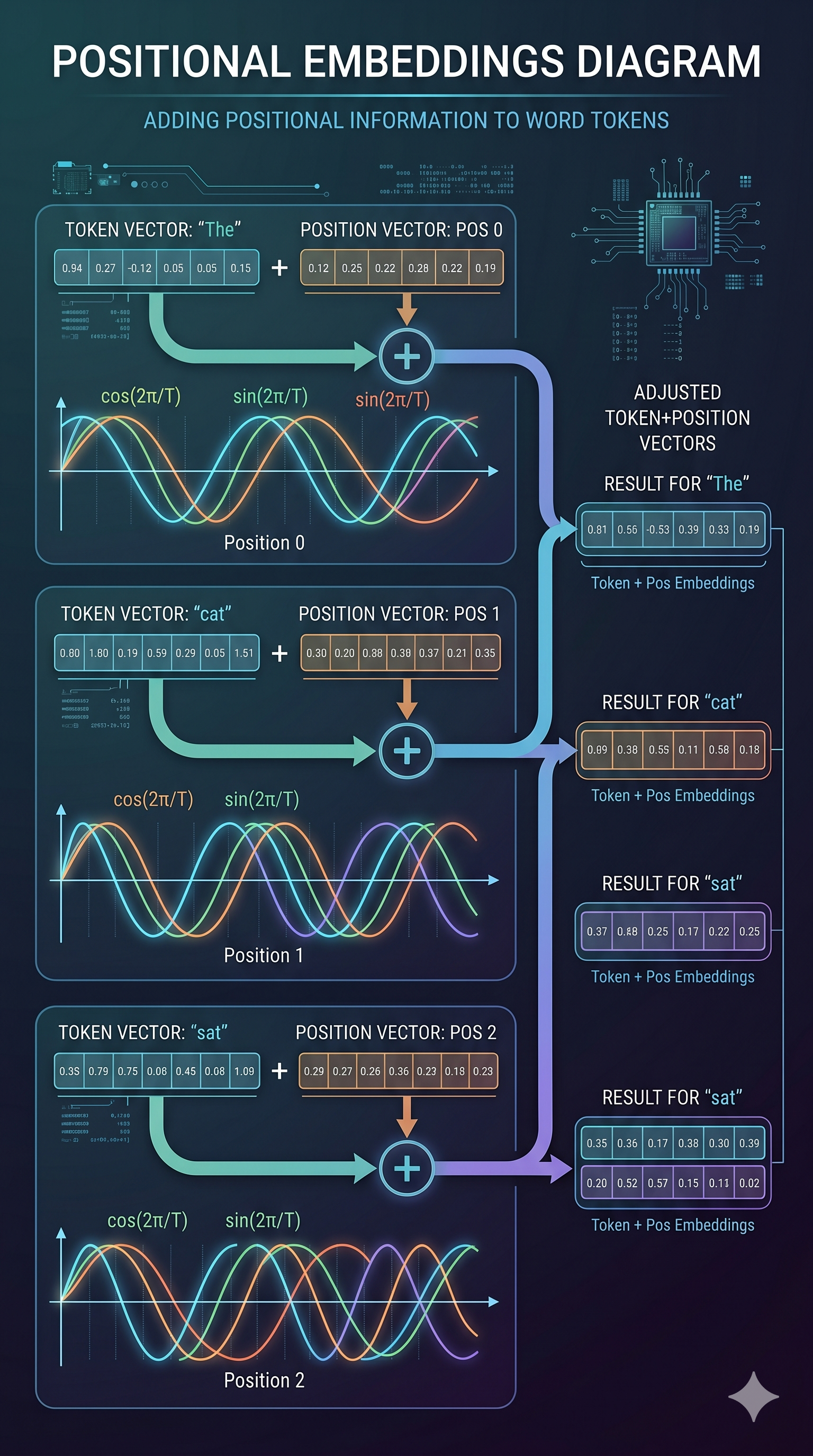
6. Positional Embeddings: Teaching the Model About Order

Here’s a problem: the embedding lookup is a table lookup. It doesn’t care that “cat” is token 2 and “sat” is token 3. Two requests with the same tokens in different orders would produce identical embeddings.

But order matters enormously. “The cat sat on the dog” and “The dog sat on the cat” have the same tokens and very different meanings.

Positional embeddings solve this by adding a position-aware vector to each token’s embedding. The model learns that “token at position 1” feels different from “token at position 5,” even if the token ID is the same.

How Is It Calculated?

There are two main approaches:

Sinusoidal (original Transformers paper): Compute a fixed sine/cosine wave pattern based on position and dimension index. Deterministic, no learned parameters.

RoPE (Rotary Position Embedding): Used by Llama, Qwen, Mistral, and most modern models. Instead of adding a vector, it rotates the query and key vectors by an angle proportional to position. The result: the dot product between two token representations naturally captures their relative distance. Elegant, and generalizes better to longer contexts than the training data.

Continuing our example. After adding positional information:

"The"  at position 0: [0.12, -0.43, 0.81] + pos(0) → [0.15, -0.40, 0.84]
" cat" at position 1: [-0.34, 0.91, 0.12] + pos(1) → [-0.31, 0.88, 0.09]
" sat" at position 2: [0.67, 0.05, -0.88] + pos(2) → [0.65, 0.03, -0.86]

The position vectors are small adjustments. Their real value is that when attention is computed later, the model can tell whether two tokens are adjacent or 200 positions apart.

CPU Bottleneck in Prefill?

Embedding lookup and positional encoding are fast operations. The real CPU bottleneck in prefill is less about these steps and more about data movement: loading the right weight tensors from CPU RAM to GPU VRAM before the transformer forward pass can begin.

For very large models that don’t fully fit in VRAM, the CPU-GPU transfer becomes the bottleneck — you’re constantly paging weight blocks in. This is why model quantization matters: a 4-bit quantized model uses less VRAM, fits entirely on GPU, and eliminates this transfer overhead. More on that in a moment.

7. The Transformer Layers: Where the Real Work Happens

After embedding + positional encoding, we have a matrix of shape [sequence_length × embedding_dim]. This matrix now passes through N transformer layers — 32 layers for Llama-3.2-3B, 80 layers for Llama-3.1-70B.

Each layer applies:

Self-attention: every token looks at every other token and decides what’s relevant
Feed-forward network (FFN): each token’s representation is independently transformed

This is where the model’s “reasoning” happens — and where most of the GPU compute goes during prefill. All tokens are processed in parallel within a layer, making prefill compute-bound. More tokens = more compute = higher TTFT.

We’ll cover the attention mechanism in detail in section 9. First, let’s see what comes out.

8. Decoding: One Token at a Time, Forever

After prefill, the model produces its first output token. Then it produces another. Then another. Each token depends on all previous tokens. This is the decode loop.

Here’s what makes decode fundamentally different from prefill: you can’t parallelize it. Token N can’t be computed until token N-1 exists. It’s inherently sequential.

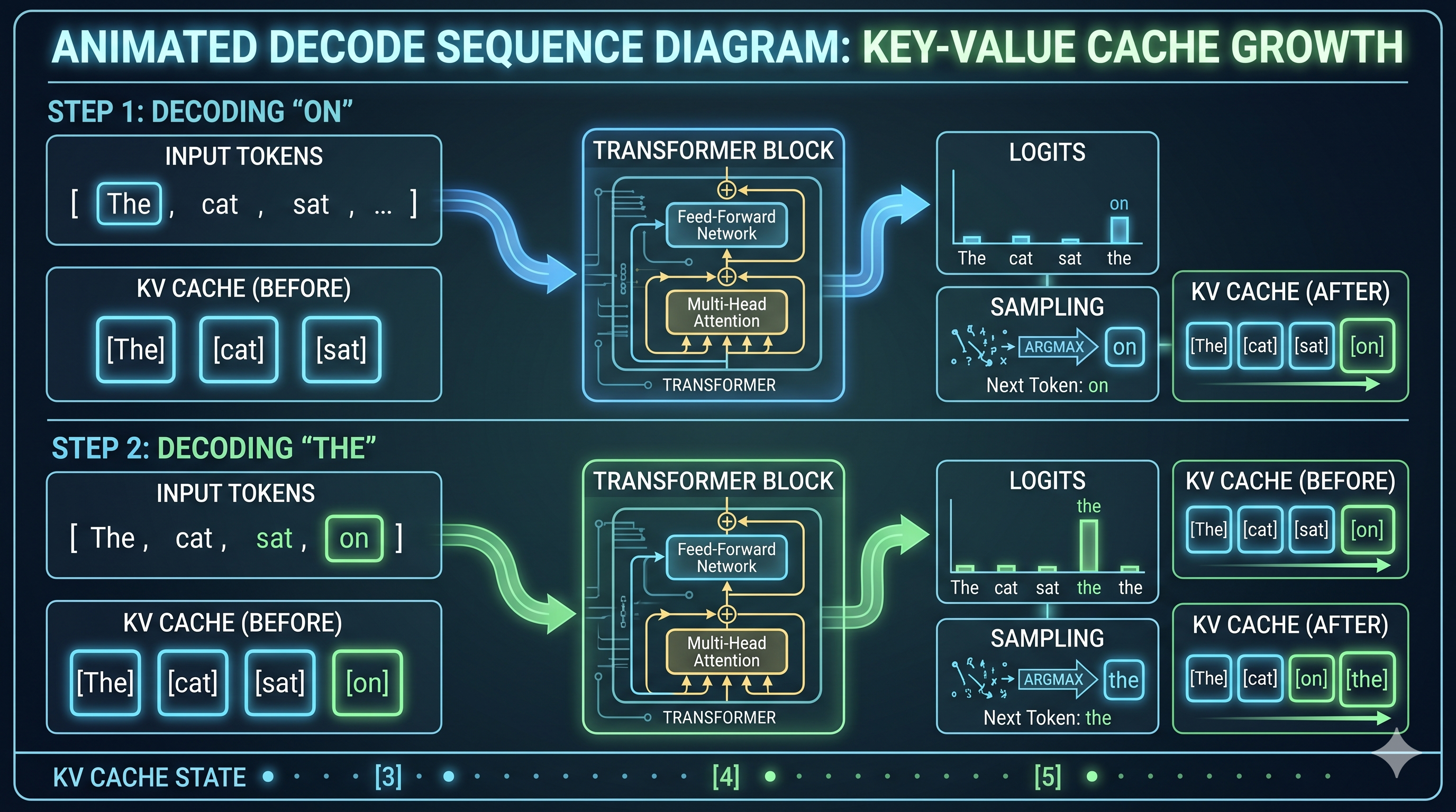
Let’s walk through two steps with our example. Our prompt was “The cat sat” and let’s say the model is going to output “on the mat.”

Decode Step 1: Predicting “on”

After prefill, we have KV cache entries for “The”, “ cat”, “ sat” (we’ll explain KV cache shortly). Now:

The model takes the last token’s representation (“ sat”) and runs it through the transformer layers
At each layer, attention is computed between “ sat” and all previous tokens via the KV cache
The final layer outputs a vector of size [vocabulary_size] — one score per possible next token. This is called the logits vector.
The logits are converted to probabilities via softmax
A token is sampled from this distribution (more below)
Result: token ID for “ on” → " on" is emitted as the first output token

KV cache: ["The", " cat", " sat"]
Current:  " sat" (last input token)
Attention: " sat" attends to "The", " cat", " sat"
Output logits: [0.001, 0.003, ..., 0.45 (" on"), ..., 0.002]
Sample: " on" ✓

Decode Step 2: Predicting “the”

Now “ on” has been generated. We add it to context:

Embed token “ on” → one new embedding vector (just one token, not the whole sequence)
Add positional embedding for position 4
Run through transformer layers, attending to KV cache for [“The”, “ cat”, “ sat”, “ on”]
Output logits → sample → “ the”

KV cache: ["The", " cat", " sat", " on"]  ← one entry added
Current:  " on" (new last token)
Attention: " on" attends to all four previous tokens
Output logits: [..., 0.67 (" the"), ...]
Sample: " the" ✓

And so it continues: “ mat” → “.” → <end> token → stop.

The Sampling Step (Where Creativity Lives)

The logits give you a probability distribution. How you sample from it is where temperature, top-k, and top-p come in:

Greedy (temperature=0): always pick the highest probability token. Deterministic. Boring for creative tasks, good for code.
Temperature > 1: flatten the distribution. More randomness, more surprising outputs, more hallucinations.
Temperature < 1: sharpen the distribution. More conservative, more predictable.
Top-k: only sample from the top K most probable tokens. Ignores the long tail.
Top-p (nucleus sampling): only sample from the smallest set of tokens whose cumulative probability exceeds p. Adaptive — sometimes that’s 2 tokens, sometimes 50.

This step is trivially cheap computationally but has enormous impact on output quality. As an SRE, you don’t usually tune this — but you will get bug reports when someone’s temperature=2.0 config makes the model output Shakespeare from a JSON API endpoint.

9. Why Memory Is the Decode Bottleneck

Here’s the thing about decode that makes it hard to optimize: on every single decode step, the model needs to run attention against all previous tokens. Not a summary of them. All of them. Via the KV cache.

For a 1000-token conversation, every decode step reads 1000 rows of KV tensors from GPU memory. For a 32-layer model, that’s 32 reads of a large tensor. For a 7B model, the KV entry for a single token at a single layer is tens of kilobytes.

The GPU’s compute cores can execute these operations fast. But they’re waiting on HBM (High Bandwidth Memory) to deliver the data. The memory bus saturates before the compute does.

The GPU is memory-bound during decode, not compute-bound.

This is why adding more CUDA cores doesn’t help decode performance as much as adding more memory bandwidth. It’s why H100s are faster than A100s for serving despite similar compute specs — the memory bandwidth jump matters more for decode than the FLOP count.

A rough intuition: during prefill, GPU utilization is high and memory is barely stressed. During decode, GPU compute is mostly idle and the memory bus is screaming.

10. KV Cache: The Most Important Data Structure in Inference

We keep mentioning the KV cache. Let’s make it concrete.

During the attention step in each transformer layer, every token produces two vectors: a Key (K) and a Value (V). These are used in attention computation: other tokens use your Key to decide how much to attend to you, and then use your Value to extract information from you.

During decode, token N needs to compute attention against tokens 1 through N-1. If we recomputed K and V for all previous tokens on every step, we’d be doing O(N²) work per decode step. That’s catastrophic.

The KV cache solves this: after computing K and V for a token, we store them. On the next decode step, we only compute K and V for the new token and look up the rest from cache.

After prefill of "The cat sat":
KV cache = {
  layer_0: { K: [k_The, k_cat, k_sat], V: [v_The, v_cat, v_sat] }
  layer_1: { K: [...], V: [...] }
  ...  (32 layers total)
}

After generating " on":
KV cache = {
  layer_0: { K: [k_The, k_cat, k_sat, k_on], V: [v_The, v_cat, v_sat, v_on] }
  ...
}
← one new entry appended per layer per decode step

The cache grows with every token generated. When the KV cache fills GPU memory:

New requests queue (they have nowhere to store their KV tensors)
Long requests get partially evicted and have to recompute (latency spike)
In the worst case: OOM crash

KV cache occupancy is the single most important resource to monitor in a serving system. It determines how many concurrent requests you can serve and how long those requests can be. When vllm:kv_cache_usage_perc starts approaching 0.9, you’re about to have a bad time.

Prefix Caching: Free Speedups

If two requests share the same system prompt, their KV cache entries for that prefix are identical. Prefix caching stores those entries once and reuses them.

In practice on my M4 Mac Mini:

Without prefix cache (cold):  TTFT 753ms
With prefix cache (warm):     TTFT 367ms
Savings:                       51% reduction in TTFT
Zero model changes required.

This is why your production system prompt should be at the beginning of every request, and why it should be identical byte-for-byte across requests. Drift in the system prompt = cache misses = higher TTFT = sad users.

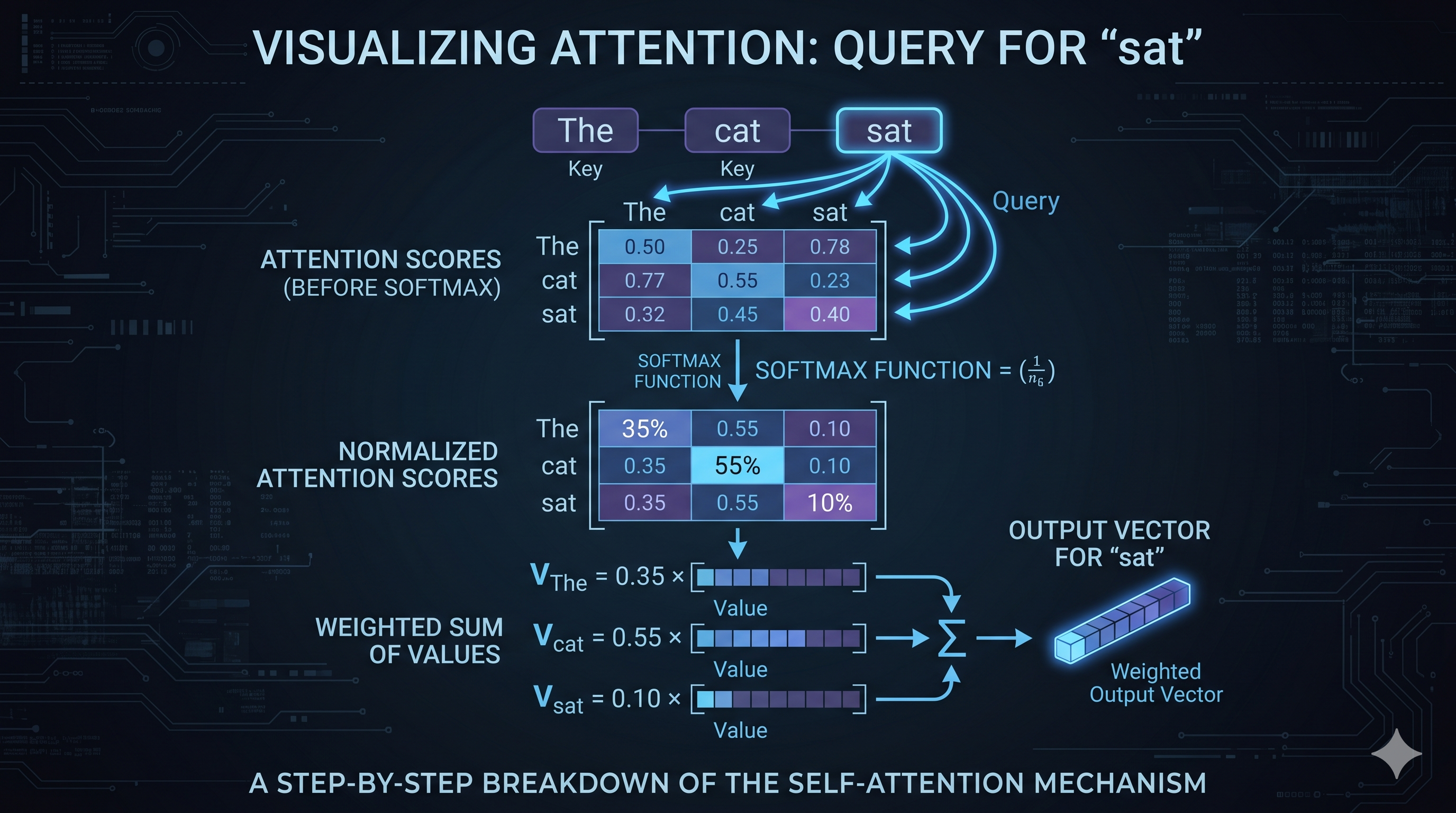
11. Attention: The Mechanism That Makes It Work

Let’s go one level deeper into what happens at each transformer layer. Attention is the core operation. Everything else is bookkeeping.

Self-Attention in Plain English

For each token, attention computes: “which other tokens should I be paying attention to, and by how much?”

It does this via three learned projections of each token’s embedding:

Query (Q): “what am I looking for?”
Key (K): “what do I offer?”
Value (V): “what information do I contain?”

For each token, you compute its dot product with every other token’s Key. High dot product = high attention score = attend more to that token. The scores are normalized via softmax, then used to weight-sum all the Value vectors.

Example with “The cat sat”:

Token: " sat"
Q_sat · K_The  = 0.8  → attend heavily to "The"
Q_sat · K_cat  = 0.9  → attend most to " cat" (makes sense)
Q_sat · K_sat  = 0.3  → attend a little to itself

Attention weights after softmax: [0.35, 0.55, 0.10]

Output = 0.35 × V_The + 0.55 × V_cat + 0.10 × V_sat

The output for “ sat” is now a blend of information from all tokens, weighted by relevance. After 32 such layers, the model has a rich, contextualized representation of every token in the sequence.

Paged Attention: Virtual Memory for KV Cache

Standard attention assumes the KV cache is one contiguous block of memory per request. This is wasteful: you have to pre-allocate the maximum possible sequence length upfront, and if the request ends early, that memory is wasted until the request completes.

PagedAttention (the key innovation in vLLM) borrows from OS virtual memory. Instead of one contiguous block, KV cache is stored in fixed-size pages (blocks) that can be non-contiguous in physical GPU memory. A page table maps logical token positions to physical blocks.

Without PagedAttention:
  Request A: [KKKKKKKKKK........] ← pre-allocated 20 slots, using 10, wasting 10
  Request B: [KKKKKK............] ← pre-allocated 20 slots, using 6, wasting 14

With PagedAttention:
  Block pool: [B1][B2][B3][B4][B5][B6][B7][B8]...
  Request A:  blocks B1, B3, B7 (non-contiguous, allocated on demand)
  Request B:  blocks B2, B4    (uses only what it needs)

The result: much higher memory utilization, more concurrent requests, less waste. Prefix cache blocks can be shared between requests with identical prefixes — only one copy of the system prompt’s KV entries needed, regardless of how many requests use it.

PagedAttention is why vLLM typically serves 2-4x more concurrent requests than a naive implementation on the same hardware.

12. Continuous Batching: The Throughput Unlock

Early inference servers were naive: accept a batch of requests, run them all through the model together, return all responses. Simple.

The problem: requests finish at different times. Short requests had to wait for long requests to complete before the next batch could start. GPU utilization looked like a sawtooth wave.

Continuous batching (also called iteration-level scheduling) fixes this. Instead of batching at the request level, the inference engine batches at the decode step level. Every iteration, it assembles the currently active tokens — some mid-generation, some just starting — into a single GPU operation.

When a request finishes, its slot is immediately available for a new request. When a new request arrives, it joins the active batch at the next iteration rather than waiting for the next batch boundary.

The result: GPU utilization stays high, latency for new requests is low, and throughput scales with the number of concurrent requests the KV cache can support — not with some fixed batch size parameter you tuned last Tuesday.

vLLM, TGI, and TensorRT-LLM all implement continuous batching. Ollama does not (as of early 2025). This is one of the primary reasons vLLM serves at 2x the throughput of Ollama under concurrent load.

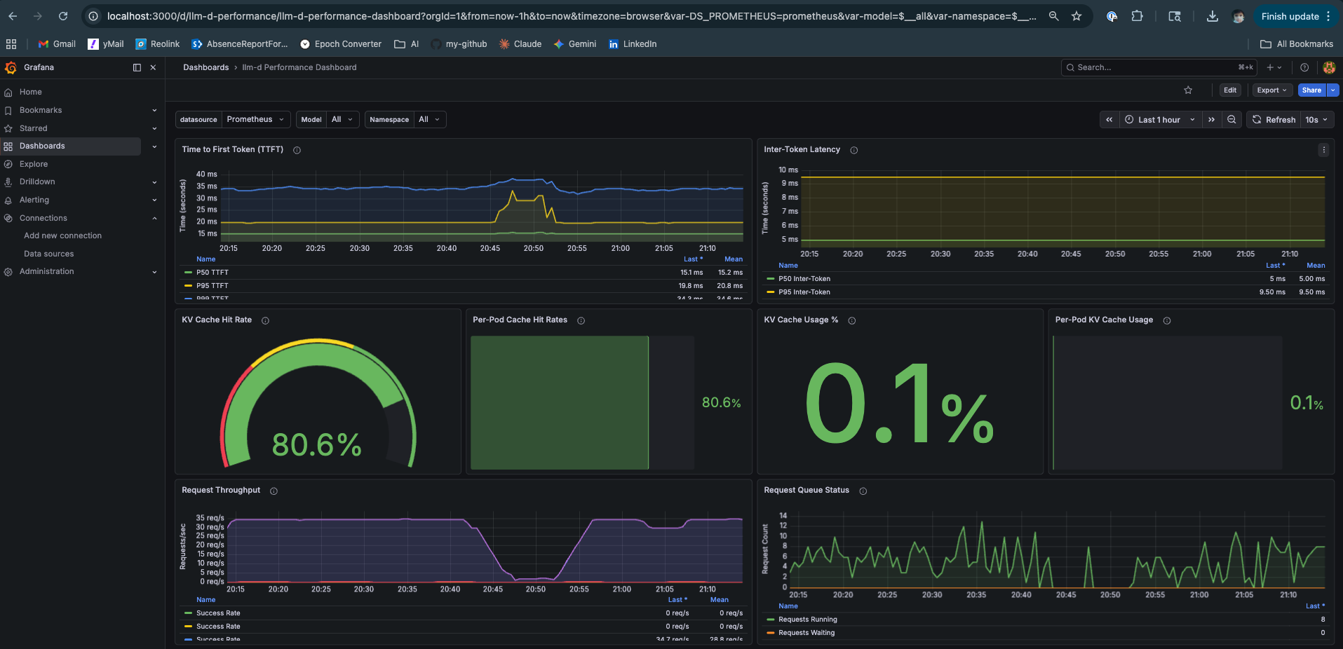
13. The Metrics That Matter

Now that you know what’s happening, the metrics become obvious rather than mysterious.

Grafana Metrics Dashboard — Real metrics from a running llm-d deployment: TTFT p50 at 15ms, ITL p50 at 5ms, KV cache prefix hit rate at 80.6% — exactly the four numbers you should have on your wall during an incident.

TTFT — Time to First Token

Definition: Wall clock time from request submission to first output token.

What it captures: Prefill time + queuing time. If your GPU is busy, TTFT absorbs the wait.

PromQL:

histogram_quantile(0.95,
  sum(rate(vllm:time_to_first_token_seconds_bucket[2m])) by (le)
)

SLO guidance: < 500ms for interactive chat. < 2s is tolerable. > 5s and users think it’s broken.

Root causes when high:

Long prompts (expected — prefill scales with length)
GPU under heavy load, requests queuing
Insufficient prefill capacity (in P/D disaggregated setups)

ITL — Inter-Token Latency (aka TPOT)

Definition: Average time between consecutive output tokens during decode. Inverse of token generation speed.

What it captures: Decode throughput per active request. Memory bandwidth is the primary lever.

PromQL:

histogram_quantile(0.95,
  sum(rate(vllm:time_per_output_token_seconds_bucket[2m])) by (le)
)

SLO guidance: < 30ms is fast, streaming feels smooth. > 100ms and you notice the typewriter effect.

Root causes when high:

Too many concurrent requests (KV cache reads competing)
Large model + small GPU memory bandwidth
KV cache approaching capacity

KV Cache Hit Ratio

Definition: Fraction of prompt tokens whose KV vectors were served from prefix cache vs recomputed.

What it captures: Effectiveness of prefix caching. High hit ratio = lower TTFT for repeated system prompts.

PromQL:

vllm:gpu_prefix_cache_hit_rate

Target: > 0.5 for most chat workloads with consistent system prompts. Near 0 means your prompts are fully unique (batch processing, no shared prefix).

KV Cache Usage

Definition: Fraction of total KV cache capacity currently occupied.

PromQL:

vllm:gpu_cache_usage_perc

Alert threshold: > 0.85. At 0.9+, vLLM starts evicting in-progress requests, causing recomputation and latency spikes. At 1.0, new requests queue entirely.

Scaling Strategy by Traffic Shape

This is where the SRE work actually lives:

Traffic Pattern	Symptom	Action
Many short prompts, many users	TTFT fine, ITL rising, KV cache full	Scale out (more replicas), or reduce `max_model_len`
Few long prompts, long outputs	TTFT high, ITL high, KV cache full fast	Larger GPU memory, or P/D disaggregation
Bursty traffic, idle baseline	P99 TTFT spikes, P50 fine	Horizontal scaling + request queuing
Consistent system prompt across requests	High TTFT on cold start only	Enable prefix caching (already default in vLLM >= 0.4)
Mixed short and long context	Unpredictable KV usage	Set per-request `max_tokens` limits strictly

The strategic insight: short prompt, many concurrent users → decode is the bottleneck, optimize for memory bandwidth and parallelism across requests. Long context, few users → prefill is the bottleneck and KV cache pressure is the constraint; P/D disaggregation helps by giving prefill its own GPU.

14. Where Does the Time Actually Go?

After running these experiments on real hardware, here’s the honest answer:

Typical inference request (short prompt, moderate load):

Tokenization:          ~0.5ms   (CPU, negligible)
Embedding lookup:      ~1ms     (GPU memory read)
Prefill (32 layers):   ~40ms    (GPU compute, scales with prompt length)
First token decode:    ~3-5ms   (GPU memory read, KV cache write)
...each subsequent token: ~3-5ms

Total TTFT:            ~45ms under no load
Total TTFT at p95:     300-500ms under load (queuing dominates)

Where load makes it worse:

Queuing before prefill starts: your request sits behind other long prefills. TTFT absorbs the entire queue wait.
KV cache contention during decode: more concurrent requests = more KV cache reads per step = higher ITL for everyone.
Memory fragmentation: without PagedAttention, wasted KV cache blocks reduce effective concurrency.

What’s predicted to improve this:

Speculative decoding: a small “draft” model generates 4-5 tokens speculatively; the large model verifies them in one forward pass. If accepted, 4 tokens for the price of ~1.5 forward passes. Reduces ITL dramatically under low concurrency, hurts at high concurrency (wasted draft compute).
P/D disaggregation: dedicated prefill GPUs handle prompt processing, dedicated decode GPUs handle generation. Eliminates the resource contention between phases. Requires fast interconnect (NVLink or RDMA) for KV transfer.
Flash Attention 3: kernel-level optimization that keeps attention computation in SRAM longer, reducing HBM reads. Already default in vLLM on H100.

15. The Inference Engines Worth Knowing

Not all inference engines are created equal, and the right tool depends on your constraints.

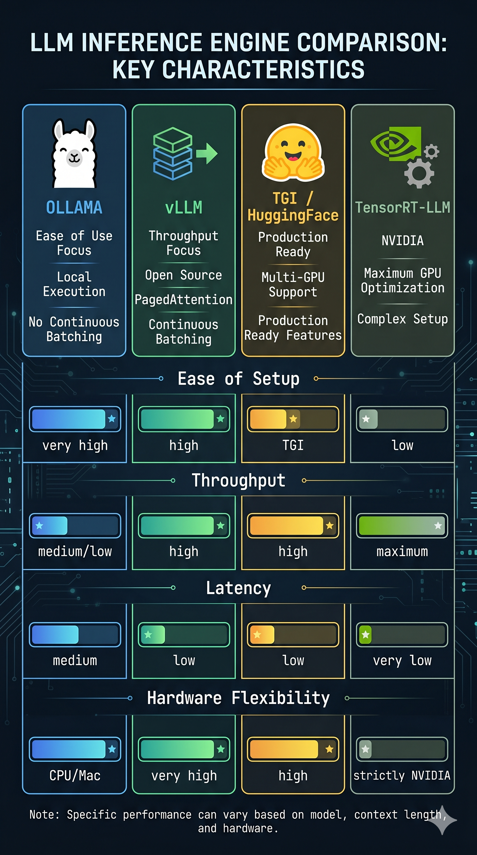
Ollama

Origin: Open source, community
Strengths: Dead simple to run, supports Apple Silicon natively, GGUF format
Weaknesses: No continuous batching (as of early 2025), worse throughput under concurrent load
When to use: Local development, single-user experiments, quick model testing
When not to use: Serving more than one user concurrently
GitHub: github.com/ollama/ollama

vLLM

Origin: UC Berkeley, now a major open-source project with significant industry contributors
Strengths: PagedAttention, continuous batching, Prometheus metrics out of the box, P/D disaggregation via llm-d
Weaknesses: More complex setup, CUDA-first (Apple Silicon support via vllm-metal is experimental)
When to use: Production serving, multi-user, research with real load
When not to use: You just want to run one model locally and don’t want to think about it
GitHub: github.com/vllm-project/vllm

TGI (Text Generation Inference)

Origin: HuggingFace
Strengths: First-class support for new HuggingFace models, FlashAttention, tensor parallelism
Weaknesses: Slower to adopt innovations than vLLM, somewhat opinionated config
When to use: You’re already in the HuggingFace ecosystem and want good defaults
GitHub: github.com/huggingface/text-generation-inference

TensorRT-LLM

Origin: NVIDIA
Strengths: Best possible performance on NVIDIA hardware, optimized kernels, inference graph compilation
Weaknesses: NVIDIA-only, complex setup, compiled engines are model+hardware-specific (can’t move them)
When to use: You have a fixed model, fixed NVIDIA hardware, and need maximum performance
When not to use: You want flexibility, you’re running experiments, or you don’t own your hardware
GitHub: github.com/NVIDIA/TensorRT-LLM

The META / Research Options

llama.cpp — github.com/ggerganov/llama.cpp: The CPU-first runtime. Runs quantized models on CPU, reasonably fast, the ancestor of Ollama.
ExLlamaV2 — github.com/turboderp-org/exllamav2: Highly optimized for RTX GPUs specifically. EXL2 quantization format is more sophisticated than GPTQ or AWQ — per-layer bit allocation instead of uniform quantization.
MLC-LLM — github.com/mlc-ai/mlc-llm: Cross-platform (compiles to CUDA, Metal, Vulkan). Good for deploying to diverse hardware.

16. The Languages Behind It All

If you open the source code of a modern inference engine, here’s what you’ll find:

Python: The top layer. API server, request handling, scheduling logic, metric collection. vLLM’s scheduler and OpenAI-compatible API are Python. This is also where most bugs live.

CUDA (C++): The performance layer. Attention kernels, memory management, GPU operations. Flash Attention is CUDA. PagedAttention’s physical block management is CUDA. If Python is the restaurant, CUDA is the kitchen.

Rust: The fast utilities layer. HuggingFace’s tokenizers library is Rust — because tokenizing millions of requests fast matters. NIXL (the KV cache transfer layer in llm-d) has Rust/C++ components. Growing presence in inference tooling.

Go: The orchestration layer. Kubernetes operators, control plane tooling, health checks, routing logic. If you’re writing infrastructure around inference — operators, routers, schedulers — Go is where the work happens.

C++ (non-CUDA): llama.cpp is pure C++ with optional CUDA/Metal backends. TensorRT-LLM has heavy C++ in the engine.

For SREs/DevOps: You live in Python (scripts, load tests), Go (operators, K8s controllers), and YAML (unfortunately). CUDA is worth being able to read — not write, just understand why a kernel fusion matters and what a grid/block size means. Rust fluency is a genuine differentiator if you want to contribute upstream.

17. What CPU vs. Memory Intensive Means, Summarized

After all of the above, here’s the clean summary of which hardware resource each step stresses:

Step	Hardware	Why
Tokenization	CPU	Text processing, hash lookups, BPE merges
Embedding lookup	GPU memory	Row lookup in large weight matrix
Positional encoding	GPU compute	Fast arithmetic, small matrix
Prefill (attention + FFN)	GPU compute	Matrix multiplications, all tokens in parallel
Decode attention	GPU memory bandwidth	KV cache read per step, memory-bound
Decode FFN	GPU compute	Weight matrix multiply per step
KV cache management	GPU memory	Allocation, paging, eviction
Sampling (logit → token)	GPU compute	Softmax + sample, fast

The pattern: prefill is compute-bound, decode is memory-bound. This is the fundamental tension that all inference optimization — P/D disaggregation, speculative decoding, PagedAttention, quantization — is ultimately trying to resolve.

18. What an SRE Actually Needs to Know

You don’t need to write CUDA. You don’t need to derive the attention formula. But you do need a mental model that lets you answer these questions in production:

Why is TTFT high? → Prefill bottleneck or queuing. Long prompts? GPU saturated?
Why is ITL degrading? → KV cache pressure. Too many concurrent requests. Memory bandwidth saturating.
Why did the GPU OOM? → KV cache exhausted. Too many long requests, no eviction headroom.
Why is throughput low? → No continuous batching. Poor concurrency config. Batch size too small.
Why does prefix caching not help? → System prompt is changing per-request. Fix the app layer.
Which GPU should I buy? → For inference: memory bandwidth matters more than FLOP count. H100 > A100 for serving not because of compute but because of HBM3 bandwidth.
Why is quantization worth it? → A 4-bit model serves faster (decode is memory-bound, smaller tensors = faster reads) and fits on cheaper hardware. Quality loss is usually acceptable.

The mental model in one sentence: LLM inference is split between a compute-hungry prefill phase and a memory-hungry decode phase, connected by a KV cache that is your most critical resource to manage.

Everything else — PagedAttention, continuous batching, P/D disaggregation, speculative decoding, quantization — is an optimization layered on top of that fundamental structure.

The Summary: A Mental Model for Production

If you’ve made it this far, you’ve realized that LLM inference isn’t magic; it’s a measurable, optimizable systems engineering challenge. The execution pipeline breaks down into three distinct phases with unique bottlenecks: Tokenization (CPU-bound), Prefill (GPU compute-bound), and Decode (GPU memory-bound).

To help you debug that 2:00 AM latency spike, here is the final synthesis of the mechanics we’ve covered:

The “War Room” Reference Table

Phase	Core Mechanism	Primary Bottleneck	SRE Metric to Watch
Ingress	Tokenization	CPU / Latency	Tokenizer Latency
Processing	Prefill	GPU Compute (FLOPs)	TTFT (Time to First Token)
Generation	Decode Loop	Memory Bandwidth	ITL/TPOT (Inter-token Latency)
State	KV Cache	VRAM Capacity	Cache Usage % & Hit Rate

The Final Principles (Your TL;DR)

Weights are Static Data: The GGUF or Safetensors file is essentially a massive, math-heavy lookup table. You aren’t executing code; you are performing matrix math against frozen numbers.
Quantization is a Free Lunch: Lowering precision (e.g., to INT4) reduces tensor size, which directly loosens the memory bottleneck during decoding, often improving throughput by 20-40%.
The KV Cache is Your Most Precious Resource: It prevents $O(N^2)$ recomputation by storing token state. Managing this via PagedAttention and Prefix Caching is what separates a toy demo from a production-grade service.
Attention is the Relationship Engine: It uses Queries, Keys, and Values to calculate which tokens matter to each other. It’s why the model understands context, but it’s also why memory pressure scales with your prompt length.
Continuous Batching is the Efficiency Unlock: By batching at the “word” level rather than the “request” level, you keep the GPU busy even when individual users have wildly different response lengths.

The ultimate constraint in scaling model serving isn’t raw compute power, but memory bandwidth and the strict management of the KV Cache. By understanding the mechanical realities beneath the hood—like PagedAttention, continuous batching, and quantization—infrastructure engineers can move past guesswork and systematically optimize for the metrics that dictate user experience: TTFT and TPOT.

Conclusion: The Field Is Moving, The Fundamentals Aren’t

The implementation details of LLM inference in 2025/2026 are changing fast enough to give you whiplash, but the underlying physics of the problem haven’t moved an inch. Prefill will always be compute-hungry. Decode will always be memory-hungry. Attention will always scale quadratically with context length unless someone breaks the math. These aren’t framework quirks; they are the mechanical realities of how transformers work.

Transitioning to LLMOps requires a fundamental shift in how we manage system state. We are no longer scaling stateless pods; we are actively managing distributed GPU memory. The engineering headroom to optimize this is enormous, and the landscape is shifting rapidly:

The model size curve is bending: Smaller, highly-optimized 7B models are now punching above the weight of older 70B giants, distributing the inference problem across a much wider variety of hardware.
The memory bottleneck is softening: Bleeding-edge KV cache compression techniques are reducing per-token memory footprint from kilobytes down to a handful of bytes, loosening the strict constraints of the decode phase.
The edge is becoming viable: As inference pushes to mobile NPUs and WebGPU, serving a 3B parameter model starts to look less like a Kubernetes workload and more like a firmware binary.

Yet, the operational reality remains unchanged. When a model is in production and serving real traffic, someone has to know why TTFT spiked at 2am, why the KV cache hit 95% utilization under Tuesday’s load, and why the p99 ITL is three times the p50.

Mastering the mechanics of inference separates a fragile AI prototype from a resilient production platform. The inference stack will keep evolving. The need for a rigorous mental model to debug it won’t.

Next up: In the next post, we’ll take these first principles and see how they dictate the architectural trade-offs behind the major inference engines: Ollama, vLLM, TGI, and TensorRT-LLM.

I’m an infrastructure engineer with 11+ years in distributed systems (D-Wave, Enbala, MasterCard, Cisco), currently going deep on LLM serving and inference optimization. This series is grounded in hands-on experiments — Mac Mini to Lambda Labs GH200 to RunPod A100 clusters. I write what I actually learned, including the parts that didn’t work.

Find me on GitHub: kraghavan

Find me on Linkedin: Karthika Raghavan

Twitter Facebook LinkedIn