In the previous post I documented everything that broke during the llm-d deployment on a Lambda Labs GH200. Ten gotchas, two false starts, one ticking hourly bill.
This post is the payoff — and more than that, it’s an attempt to say something useful beyond “look at these numbers.” The numbers are good. But the more interesting question is what they reveal about inference architecture that applies regardless of which GPU you’re running on or which serving framework you’ve chosen.
Hardware: Lambda Labs GH200 480GB, ARM64
Model: Qwen/Qwen3-0.6B
Stack: llm-d v0.4.0, vllm/vllm-openai:latest, Istio gateway, kube-prometheus-stack
Load testing: Locust with tenant simulation
Observability: Prometheus + Grafana (llm-d Performance Dashboard, llm-d vLLM Overview)
The Hardware Deserves More Than a Footnote
Most inference benchmarks treat hardware as a footnote — “tested on an A100” — without explaining why the hardware choice matters architecturally. The GH200 is worth understanding properly because it represents a design direction that the industry is converging on, and it changes some assumptions about what’s possible in inference.
One quick note before the specs: the GH200 is technically a unified memory architecture — just like the M4 Mac Mini from the previous post. CPU and GPU share the same address space without copying data between them. The Mac Mini has 16GB at roughly 200 GB/s. The GH200 has 576GB at up to 4,000 GB/s.
The GH200 is technically unified memory — just like the M4 Mac Mini. One costs $799. The other costs $2.29 per hour and will make you feel considerably better about your Mac Mini purchase. Same architectural principle, considerably different ambitions — and as the numbers in this post will show, considerably different outcomes.
Grace Hopper — One Package, Two Chips, One Memory Bus
The GH200 is not a GPU. It’s a Grace Hopper Superchip — NVIDIA’s Grace CPU (72 ARM Neoverse V2 cores) and an H100 Hopper GPU die, connected on the same package via NVLink-C2C (chip-to-chip).
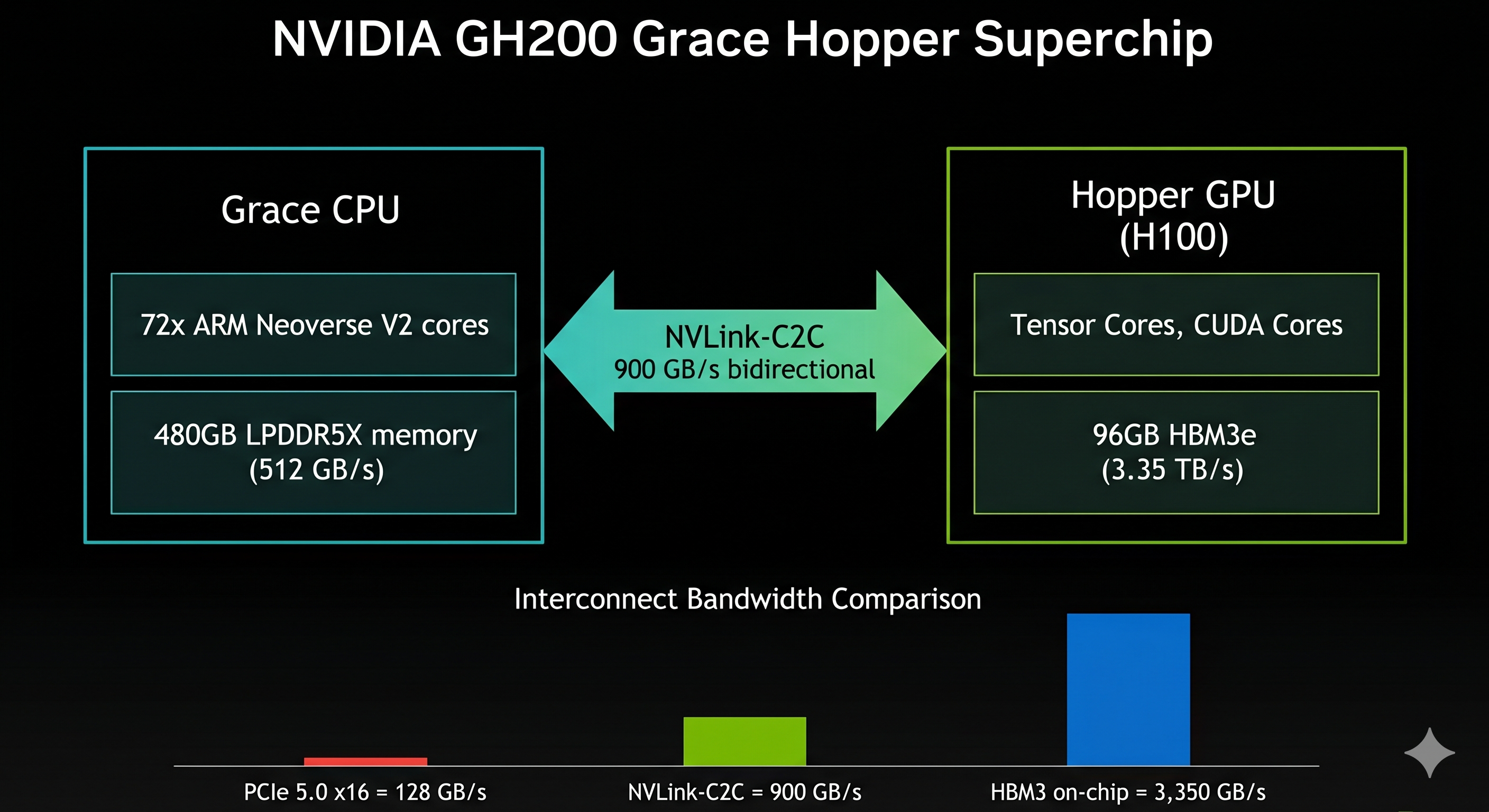
The critical number is the NVLink-C2C bandwidth: 900 GB/s bidirectional. For context:
Interconnect              Bandwidth
──────────────────────────────────────────────
PCIe 5.0 x16 (discrete)   128 GB/s
NVLink-C2C (GH200)         900 GB/s    ← 7× faster than PCIe Gen5
HBM3e on-chip (GH200)    4,000 GB/s
LPDDR5X (Grace CPU)        512 GB/s
Source: NVIDIA GH200 Grace Hopper Superchip product page and GH200 architecture whitepaper. The 7× PCIe Gen5 figure is NVIDIA’s own stated specification — “NVLink-C2C delivers up to 900 GB/s total bandwidth. This is 7x higher bandwidth than x16 PCIe Gen5 lanes.”
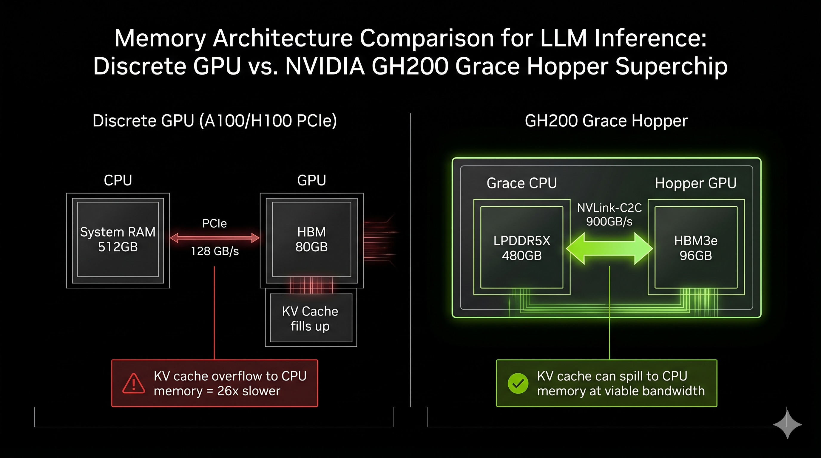
On a conventional discrete GPU system — an A100 or H100 in a PCIe slot — the CPU and GPU have separate memory pools connected by a 128 GB/s bus. Moving data between them is expensive. The GPU can’t efficiently use CPU DRAM for KV cache overflow because the PCIe bandwidth is 31× slower than the GPU’s on-chip HBM bandwidth (4,000 ÷ 128 = 31.25×). Any spill to CPU memory becomes a bottleneck.
On the GH200, the Grace CPU’s 480GB of LPDDR5X memory is accessible to the Hopper GPU at 900 GB/s over NVLink-C2C. That’s not as fast as on-chip HBM3e, but it’s fast enough to be genuinely useful. The result is a unified addressable memory space — the GPU sees up to 576GB total (96GB HBM3e + 480GB LPDDR5X) — at bandwidths that make overflow to CPU DRAM a viable architectural choice rather than a last resort.
Why This Matters for LLM Inference
At scale, inference systems are typically memory-bandwidth bound, not compute bound. This isn’t universal — small models at low concurrency can be compute-bound during prefill, and some workloads shift the bottleneck elsewhere. But for production multi-tenant serving, the binding constraint is almost always memory: how fast the hardware can load model weights and KV cache tensors for each forward pass. Every decode step reads the full KV cache. On a 7B model with a 4K context window and 32 concurrent requests, that’s dozens of gigabytes moving through the memory subsystem per second — and the rate of that movement, not the number of CUDA cores, determines your throughput ceiling.
The GH200’s NVLink-C2C doesn’t solve this — HBM3e is still the primary memory bandwidth for active inference. But it changes the economics of KV cache management. Tiered KV storage (hot blocks in HBM, warm blocks in LPDDR5X, cold blocks evicted to NVMe) becomes viable in a way it isn’t on PCIe-connected systems. llm-d’s architecture diagram from the previous post already shows tiered KV cache offloading as a first-class feature — the GH200 is the hardware that makes that design practical.
For these experiments, we didn’t exercise KV cache tiering. The model is small and the cache pressure is low. But the architecture is there, and it’s why the GH200 was the right choice for running the full llm-d stack rather than a conventional discrete GPU setup.
One Mental Model Before the Numbers
Before looking at a single metric, here is the frame I’d encourage you to carry into any inference system analysis:
LLM inference is a memory scheduling problem that looks like a compute problem.
Every team I’ve seen optimise inference focuses first on compute — GPU utilization, batch size, model quantization. These matter. But the real leverage is in memory: how much of the KV cache is warm, how often prefill recomputation is avoided, how well the scheduler keeps the right data in the right tier. The system that wins at scale is the system that does the least unnecessary work — and unnecessary prefill recomputation is the biggest source of waste in multi-tenant inference.
This is what EPP prefix cache routing is solving. Not “make the GPU faster.” Make the system do less work.
What These Experiments Actually Test
Experiments 1–4 use the inference-scheduling guide from the llm-d repo. This deploys a single decode pod that handles both prefill and decode — aggregated serving. The values.yaml is unambiguous:
prefill:
  create: false   # one pod does everything
The architecture is:
Every request →  Istio Gateway
                      │
                      ▼
                 EPP (Endpoint Picker Plugin)
                 ┌────────────────────────────────┐
                 │  prefix-cache-scorer           │
                 │  queue-depth-scorer            │
                 │  kv-utilization-scorer         │
                 └────────────────────────────────┘
                      │
                      ▼
               Single vLLM decode pod
               (prefill + decode, one process)
               KV cache lives here
With one pod, there is no cross-pod routing decision to make. The EPP’s job here is narrower: route requests with matching prefix hashes back to this pod consistently, so its KV cache stays warm. Round-robin with one pod is also consistent routing — but a naive load balancer doesn’t know about prefix hashes, so it can’t make cache-aware decisions when you add a second pod later.
What this experiment answers: Does EPP prefix-cache-aware routing actually maintain high cache utilization under realistic multi-tenant load? Does the system hold TTFT stable as concurrency grows?
What it doesn’t answer yet: What happens when you separate prefill and decode onto dedicated pods. That’s the next post.
This single-pod result is the baseline. Everything in the P/D disaggregation post gets measured against what we establish here.
The Load Test — Simulating Multi-Tenant Traffic
The Locust script simulates two traffic types in a 4:1 ratio:
# llmd-locust.py
MODEL = "Qwen/Qwen3-0.6B"

# Three tenant personas — each with a distinct long system prompt
TENANTS = [
    "You are a financial analyst assistant specializing in market data. " * 5,
    "You are a DevOps engineer assistant specializing in Kubernetes and CI/CD. " * 5,
    "You are a data scientist assistant specializing in ML pipelines. " * 5,
]

class LLMDUser(HttpUser):
    wait_time = between(0.5, 2)

    def on_start(self):
        self.tenant_prompt = random.choice(TENANTS)  # sticky for session

    @task(4)
    def tenant_request(self):
        # Repeat system prompt → cache hit opportunity
        self.client.post("/v1/chat/completions", json={
            "model": MODEL,
            "messages": [
                {"role": "system", "content": self.tenant_prompt},
                {"role": "user", "content": random.choice([
                    "Summarize the key points.",
                    "What should I focus on?",
                    "Give me 3 recommendations.",
                ])}
            ],
            "max_tokens": 80,
        }, name="tenant_session")

    @task(1)
    def cold_request(self):
        # No system prompt → cold cache, no prefix benefit
        self.client.post("/v1/chat/completions", json={
            "model": MODEL,
            "messages": [{"role": "user",
                          "content": f"Question {random.randint(1,1000)}"}],
            "max_tokens": 50,
        }, name="cold_request")
The design is deliberate. Each simulated user picks a tenant persona at startup and sticks with it — the same ~200-token system prompt on every request. This is representative of real multi-tenant SaaS inference: each customer has a system prompt that defines their product’s persona, and it’s identical on every call. The cold_request tasks (1 in 5) have no system prompt and get no cache benefit — they’re the baseline comparison within the same run.
Requests travel the full path: Mac → SSH tunnel → kubectl port-forward → Istio gateway → EPP → vLLM pod. No shortcuts.
The Results
Locust — 26,826 Requests, Zero Failures
Hardware:  GH200 480GB (single decode pod, aggregated serving)
Model:     Qwen/Qwen3-0.6B
Rate:      32 req/s sustained

Task              Requests    Failures   p50    p95    p99    avg
───────────────────────────────────────────────────────────────────
cold_request      5,450       0 (0%)     200ms  270ms  280ms  207ms
tenant_session    21,376      0 (0%)     260ms  330ms  350ms  273ms
───────────────────────────────────────────────────────────────────
Aggregated        26,826      0 (0%)     260ms  330ms  350ms  260ms
Zero failures across 26,826 requests. p99 at 350ms. The system didn’t flinch.
The comparison that matters — same Locust script structure, same traffic intent, from the Mac Mini post:
Mac Mini vLLM (5 users, 3:1 short/long):
  short prompt p50:   1,900ms
  long prompt  p50:  31,000ms
  TTFT P99:          ~7,000ms under load

llm-d on GH200 (tenant simulation, 4:1 tenant/cold):
  tenant_session p50:   260ms    ← 7.3× faster at median
  cold_request   p50:   200ms
  TTFT P99:              34ms    ← ~200× better tail latency
The gap is real, but it deserves honest attribution. Part of it is raw hardware — a GH200 is not an M4 Mac Mini. Part of it is the serving stack — llm-d with EPP routing vs vanilla vLLM. And part of it is the traffic shape — these aren’t identical experiments. What the numbers establish is a clear direction: hardware matters, but the serving architecture amplifies or squanders what the hardware can do.
What Grafana Showed
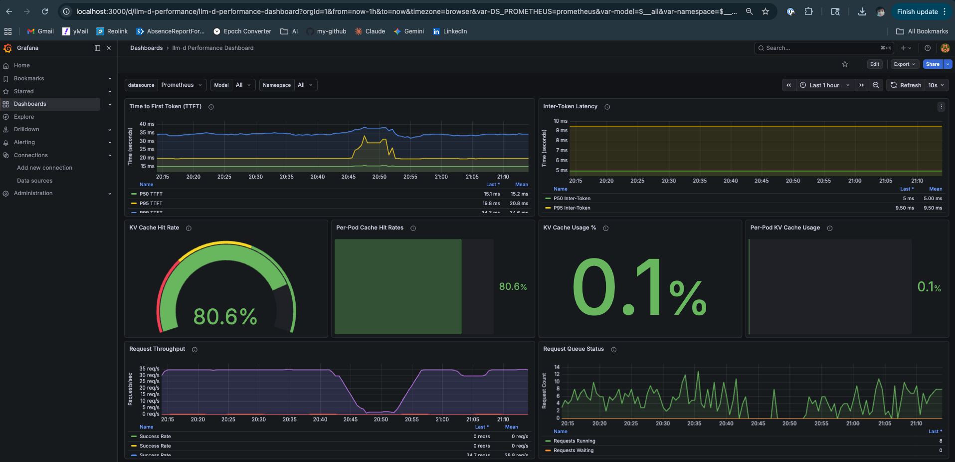
The Performance Dashboard — Read This One First
Three numbers worth pausing on:
TTFT p50 at 15ms, flat under load. The Mac Mini showed TTFT climbing past 2 seconds at p50 and 7 seconds at p99 under comparable concurrency. Here it stays at 15ms throughout. This is not just hardware — it’s what happens when 80% of your requests skip prefill entirely because their KV blocks are already warm. The system is doing less work per request on average, which is why latency stays stable as concurrency grows.
A common mistake in inference optimisation is treating TTFT stability as a tuning parameter — something you achieve by adjusting batch sizes, memory utilization settings, or scheduler parameters. It isn’t. TTFT stability under load is an architectural property. It follows from having enough cache hit rate to keep the average prefill cost low. Once cache hit rate drops below ~50%, no amount of tuning recovers the tail latency. The right intervention is upstream: better routing, larger KV cache budgets, or separation of prefill and decode workloads.
KV Cache Hit Rate at 80.6%. This is the single most actionable metric in multi-tenant inference. It tells you how much work the system is not doing. At 80.6%, roughly 4 in 5 tenant requests reuse cached KV blocks and skip prefill recomputation. The inverse is the expensive number: 19.4% of requests are cold — those are full prefill operations. In a system with 100 GPU-hours of work per day, improving cache hit rate from 80% to 90% saves 10 GPU-hours. That’s not a performance metric. That’s a cost metric.
ITL at 5ms. Inter-Token Latency is the gap between consecutive tokens during decode — a direct measure of decode throughput. At 5ms per token, that’s 200 tokens per second per request. More importantly it’s flat — it doesn’t increase as the test runs, which confirms there’s no memory pressure or scheduler thrashing affecting the decode phase. When ITL climbs under load, it’s usually a sign that the KV cache is filling and evictions are occurring. Here it’s not.
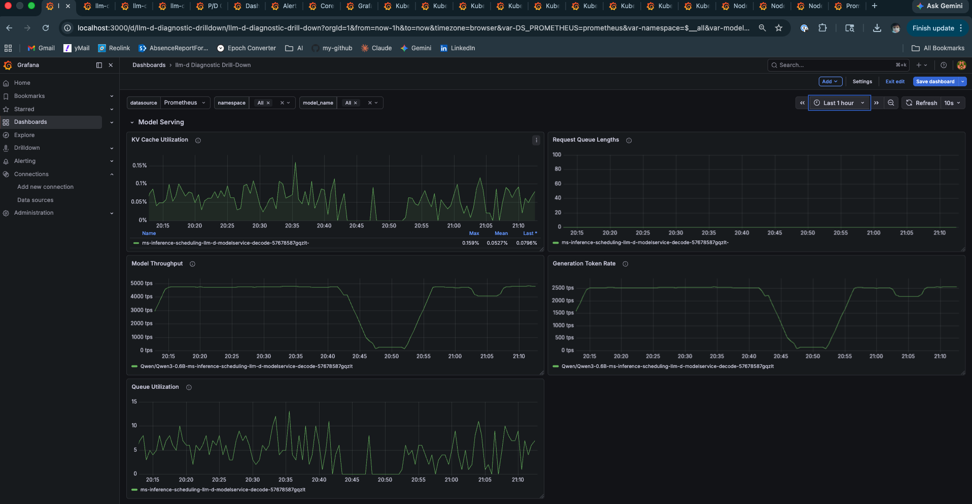
Prefix Cache Hit Rate — The Number Behind the Number
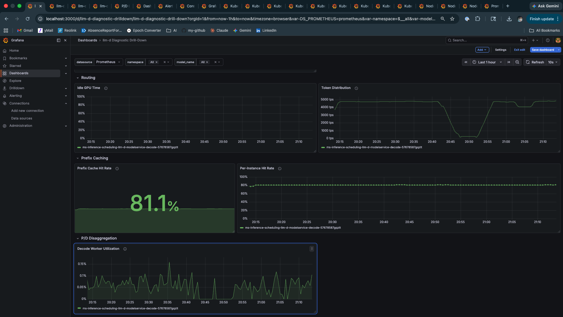
The 81.1% gauge is the aggregate. The Per-Instance time series at 80% is the more meaningful signal — it shows the cache was warm within the first few minutes and held that level for the entire test duration. This is what stable prefix cache routing looks like: not a spike that decays, but a plateau that holds.
What this means at scale: At three tenant profiles with ~200-token system prompts, 81% cache hit rate is achievable on a single pod with a small model. As you scale to 50 tenants, 500, or 5000, the picture changes. The working set of system prompts grows beyond what a single pod’s KV cache can hold. Cache hit rate degrades. TTFT rises. This isn’t a failure of EPP routing — it’s a KV cache capacity problem, and the architectural response is either larger KV budgets per pod, more pods with affinity-based routing, or tiered KV offloading. The GH200’s NVLink-C2C is exactly the hardware that makes that third option viable. This experiment doesn’t exercise it. The architecture supports it.
E2E Latency and Scheduler State
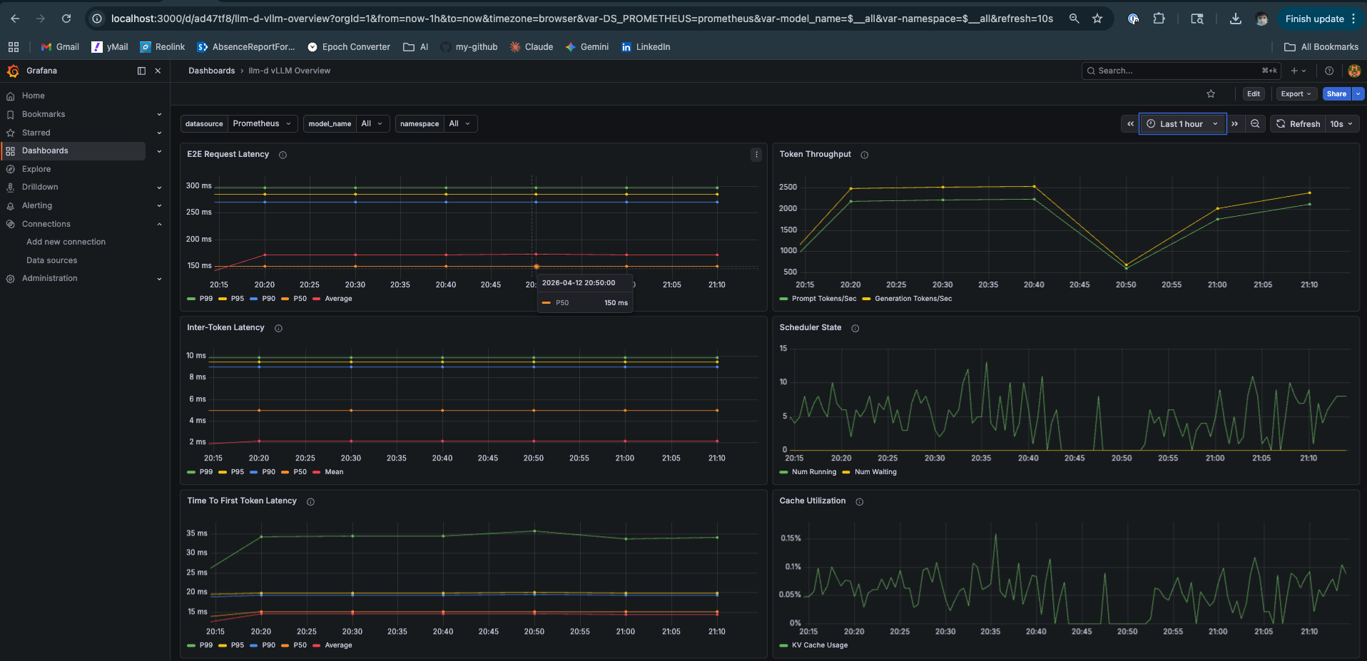
The Scheduler State panel deserves attention. Num Running is the active batch size — how many sequences share a GPU forward pass. Num Waiting is the queue depth. Both staying low and flat means continuous batching is absorbing load without queuing. Compare this to the Mac Mini Locust test where Num Waiting spiked to 5 and TTFT degraded proportionally.
Cache Utilization at 0.15% is a function of model size. Qwen3-0.6B at this concurrency level barely touches the KV pool. The same test with Llama-3-8B would show a fundamentally different curve — and that’s where the GH200’s memory architecture starts mattering in ways that go beyond raw numbers.
Prefill vs Decode — The Two-Phase Separation Made Visible
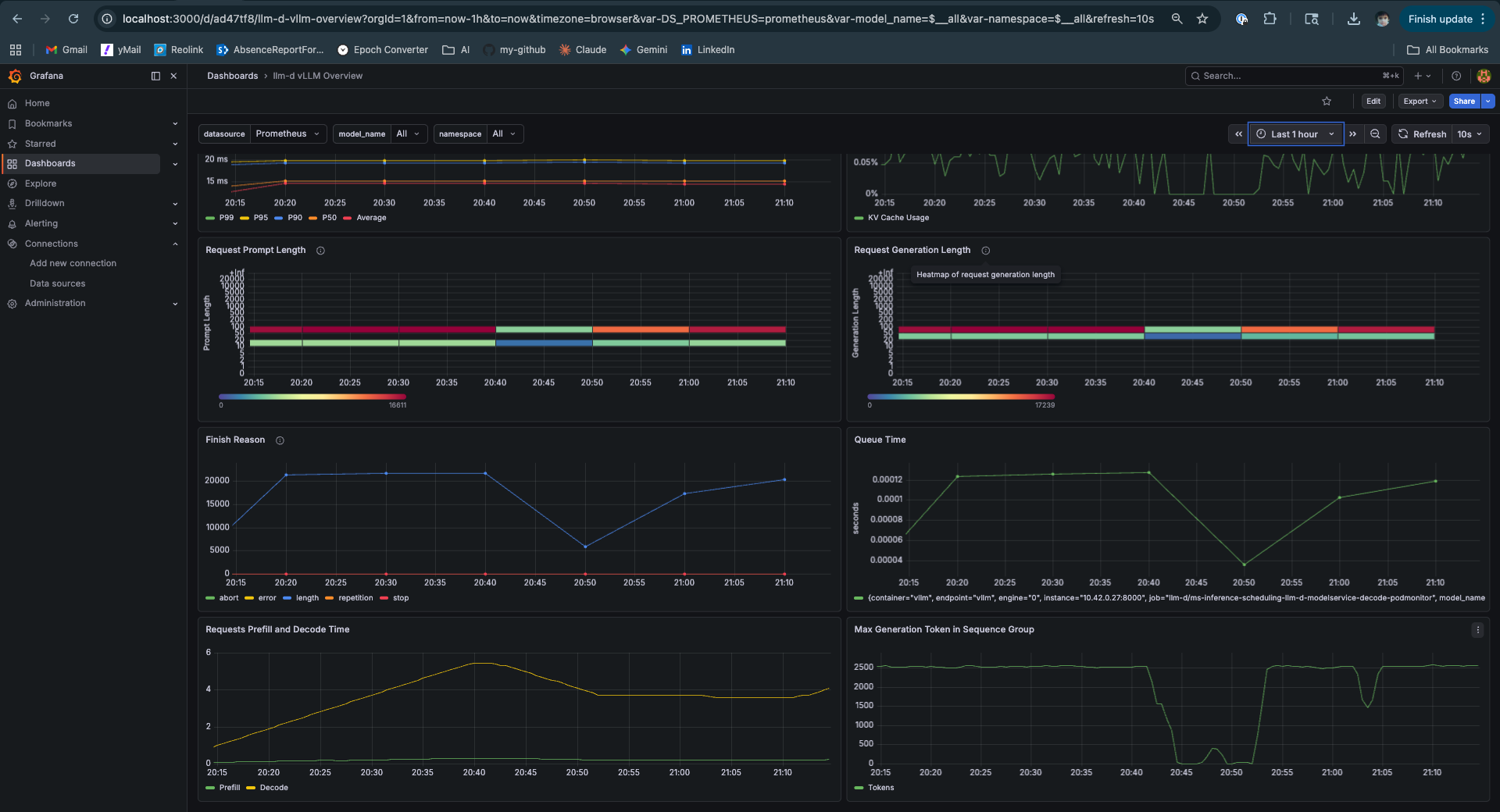
This panel is the most architecturally revealing one in the dashboard. The yellow prefill line and the green decode line on the same chart, from the same pod, tell you everything about why P/D disaggregation exists.
Prefill is compute-bound and bursty. Its cost scales with prompt length. It spikes when a cold request arrives. Decode is memory-bandwidth-bound and steady. Its cost scales with the number of tokens being generated. On the same pod, every prefill spike steals GPU time from active decode sequences — those sequences stall mid-generation while the prefill runs.
In a disaggregated setup, the yellow line comes from a prefill pod pool and the green line from a decode pod pool. Prefill spikes are isolated. Decode runs uninterrupted. TTFT for long prompts no longer delays short prompts waiting in the decode queue.
Here those lines share a pod. The system works well at this scale and concurrency — the numbers prove it. But the architectural tension is visible in the chart. That’s what the next post is about.
TTFT P99 — The Warmup Signature
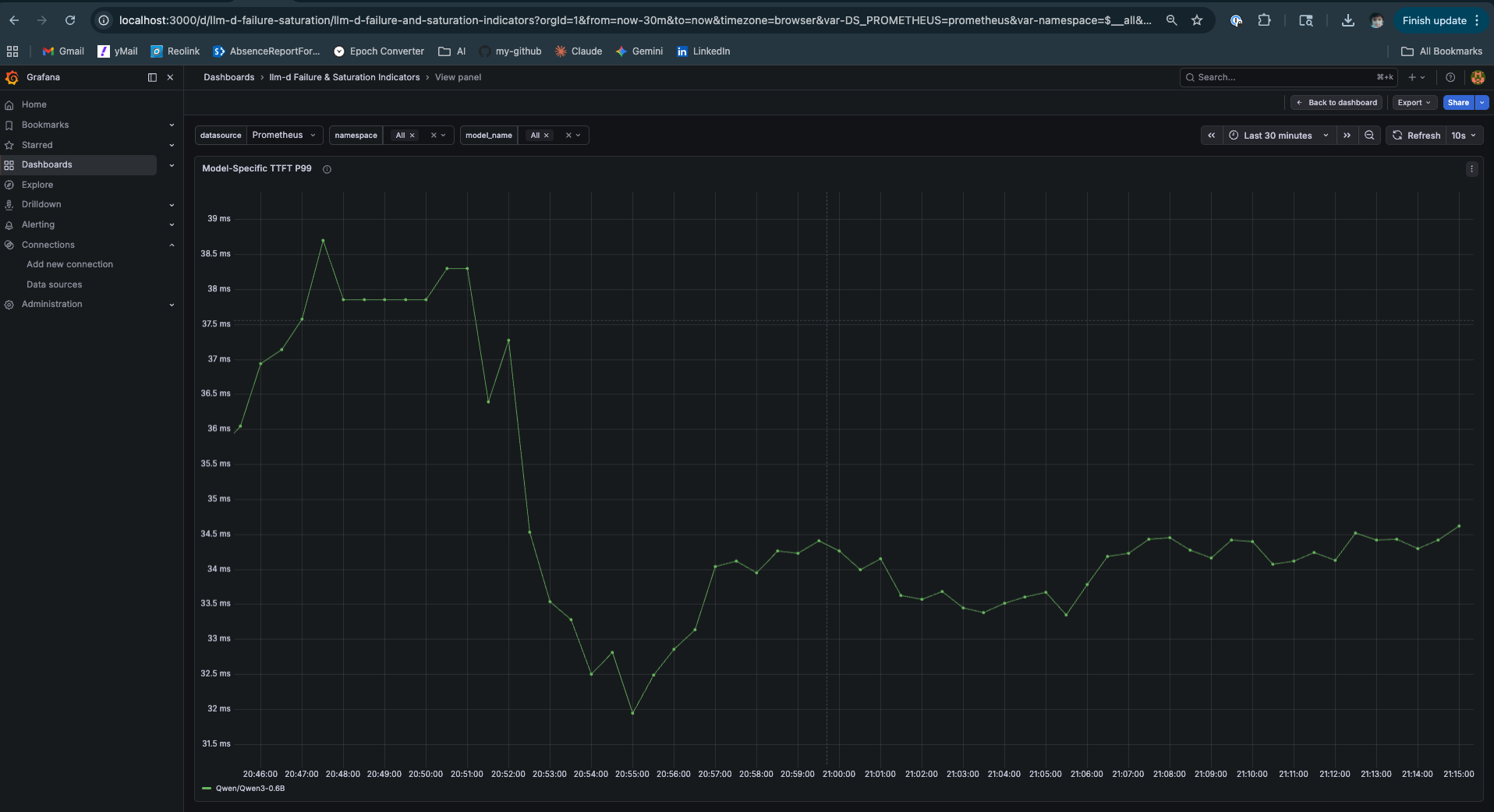
TTFT P99 dropping from 39ms to 32ms and then holding at 34ms is the cache warmup signature in the tail. The first requests from each tenant session are cold — full prefill. As sessions accumulate, KV blocks warm, and the P99 reflects that. The key signal is the plateau: P99 stops dropping once the cache is warm and doesn’t creep upward under sustained load. This is a system that has found equilibrium.
Model Throughput and Queue State
Model Throughput at 4,000–5,000 tokens per second is what a GH200 looks like under moderate load with a small model. The brief Queue Utilization spikes that drain immediately are continuous batching doing its job — burst arrivals get absorbed into the current decode step rather than queuing. This is the architectural behaviour that separates vLLM from naive sequential servers.
The Complete Benchmark Reference
Hardware:  Lambda Labs GH200 480GB (Grace Hopper)
Model:     Qwen/Qwen3-0.6B
Stack:     llm-d v0.4.0, single decode pod (prefill: create: false)
           EPP: prefix-cache-scorer + queue-scorer + kv-utilization-scorer

─── Locust ───────────────────────────────────────────────────────────
  Total requests:   26,826     Failures:    0 (0%)
  Sustained rate:   32 req/s

  Task             p50    p95    p99    avg    req/s
  tenant_session:  260ms  330ms  350ms  273ms  25.5
  cold_request:    200ms  270ms  280ms  207ms   6.5
  Aggregated:      260ms  330ms  350ms  260ms  32.0

─── Grafana — Performance Dashboard ──────────────────────────────────
  TTFT p50:                 15ms
  TTFT p95:                 19ms
  TTFT P99 (settled):       ~34ms
  ITL p50:                  5ms   (≈ 200 tok/s)
  ITL p95:                  9.5ms
  KV Cache Hit Rate:        80.6% (gauge) / 81.1% (drill-down)
  Request Throughput:       28.8 req/s
  Model Throughput:         4,000–5,000 tps peak
  Cache Utilization:        0.15%

─── vs Mac Mini (Post 2, same script structure) ──────────────────────
  tenant p50:  Mac Mini 1,900ms  →  GH200 260ms   (7.3× faster)
  TTFT P99:    Mac Mini ~7,000ms →  GH200 34ms    (~200× better)
What This Proves — and What It Doesn’t
What it proves:
EPP prefix cache routing achieves 81.1% cache hit rate under realistic multi-tenant load. That’s not a configuration artifact — it’s the result of the EPP scoring prefix hashes and routing tenant sessions to the pod holding their warm KV blocks. The system holds TTFT at 15ms p50 and 34ms p99 under 32 req/s sustained, with zero failures.
More broadly: in multi-tenant inference systems with repeated system prompts, cache hit rate is typically the highest-leverage optimisation variable. GPU utilization, batch size, and quantization all matter — but they reduce the cost of work the system is already doing. Cache hit rate determines how much work gets skipped entirely. At 81%, the system is doing roughly 5× less prefill work than a round-robin deployment that scatters the same tenant’s requests across pods with cold caches. That ratio is hard to match through hardware improvements alone.
What it doesn’t prove:
This is a single pod, a small model, and three tenant profiles. The working set fits comfortably in the KV cache — hence 0.15% utilization. Real multi-tenant deployments have hundreds or thousands of tenant profiles. As the working set grows, cache hit rate degrades. The EPP routing remains correct, but the pod’s KV cache can’t hold every tenant’s prefix simultaneously. The responses to that problem — larger KV allocations, more pods with affinity routing, tiered KV offloading to the GH200’s LPDDR5X — are architectural decisions that require knowing the working set size and access pattern distribution. This experiment establishes that the routing mechanism works. Capacity planning is a separate problem.
What Most Teams Get Wrong
Most inference optimisation work focuses on the supply side — faster hardware, more efficient models, better batching. This is necessary but insufficient. The demand side — how requests are shaped and routed before they reach the GPU — is where the real leverage lives at scale.
The dominant optimisation lever depends on where your system actually sits. Before reaching for more hardware, diagnose the bottleneck:
| Scenario | Primary Bottleneck | Highest-Leverage Fix |
|---|---|---|
| Low cache hit rate (<50%) | Prefill recomputation | Routing + request shaping |
| High cache hit, low utilization | Scheduling inefficiency | Continuous batching config |
| High utilization, rising latency | Memory bandwidth | Better hardware / parallelism |
| High working set (many tenants) | KV cache capacity | Tiered cache / pod sharding |
Most teams misdiagnose their bottleneck and optimise the wrong layer. A team with a 30% cache hit rate buying faster GPUs is solving the wrong problem — they’ll run twice as fast through twice as much unnecessary prefill work. The 81% cache hit rate in these experiments means the system is doing roughly 5× less prefill than a naive round-robin deployment on identical hardware. No GPU upgrade achieves that ratio. Routing does.
The practical entry point: instrument your cache hit rate first. If it’s below 50%, the fix is upstream — consistent system prompts, session-affinity routing, and a scheduler that knows about prefix hashes. Hardware comes after you’ve exhausted the routing lever.
A non-obvious failure mode: high aggregate cache hit rate masking per-tenant unfairness.
A subtle failure appears when cache hit rate is high but unevenly distributed across tenants. If a small number of tenants dominate traffic, their KV blocks stay hot while long-tail tenants constantly miss the cache. The system reports a healthy aggregate hit rate — 80%, 81% — but tail latency degrades because cold tenants always pay full prefill cost.
This leads to a misleading conclusion: “the cache is working.” In reality, the system is biased toward high-frequency tenants. The aggregate metric looks healthy precisely because the popular tenants pull it up — while every new or low-frequency tenant experiences the system as if caching doesn’t exist.
In these experiments, three tenant profiles at similar frequencies produced clean aggregate numbers. Production systems with hundreds of tenants and a power-law access distribution will not. Fixing uneven cache efficiency requires either per-tenant cache accounting to surface the distribution, or explicit isolation of long-tail traffic to prevent it from competing with high-frequency prefixes for the same KV blocks. Without this, cache efficiency improves averages while silently degrading fairness — which is the kind of problem that shows up in p99 SLA breaches, not in dashboard summaries.
Connecting the Dots Across This Series
This series started on an M4 Mac Mini with a 400MB model and a Python script measuring TTFT. It’s worth pausing to trace what the numbers across all three posts are actually saying — because they’re saying the same thing at different scales.
Post 1 established the theory: decode is memory-bandwidth bound. Prefill competes with decode for the same resources. KV cache management is the central architectural problem in inference. These aren’t vLLM-specific observations — they’re properties of the transformer architecture itself. They hold on any hardware, any framework.
Post 2 ran two experiments on identical hardware. Ollama vs vLLM on the same M4 chip, same unified memory, same model family. The result — 14,062ms vs 6,543ms p50, 2.15× faster — had nothing to do with the hardware. Ollama processes requests sequentially. vLLM uses continuous batching. Same silicon, 2× throughput difference from a software architecture decision. That result matters because it isolates the variable: serving architecture, not hardware.
Then under load, even vLLM on the Mac Mini hit the ceiling. Long prompts drove TTFT to 31 seconds at p50. The Mac Mini’s 16GB unified memory pool — shared between model weights, KV cache, and OS — ran out of headroom. The principle from Post 1 materialised as a real number: when the KV cache competes for the same memory as the model weights, concurrency suffers.
This post added two more variables: real GPU hardware and intelligent routing. The GH200 with NVLink-C2C at 900 GB/s changes the memory economics — the GPU can address 480GB at viable bandwidth, not just 16GB. EPP prefix cache routing adds the third variable: the system avoids prefill work entirely for 81% of requests by keeping KV blocks warm.
The result is 260ms p50 and 34ms P99 at 32 req/s. But attributing that entirely to the GH200 would be wrong — and that’s the point. The Ollama experiment on the Mac Mini already proved that hardware alone doesn’t determine the outcome. The GH200 sets a much higher ceiling. EPP routing determines how close you get to it.
The through-line: hardware sets the ceiling. Serving architecture determines how close you get to it. This has been true at every scale in this series — a $0 Mac Mini, a $2.29/hr GH200, and everything in between. The engineers who understand this spend their optimisation budget on routing and request shaping first, and on hardware second. The engineers who don’t buy more GPUs and wonder why the numbers don’t improve proportionally.
What Comes Next
The prefill vs decode time panel in this post showed two lines on the same chart — prefill varying with cache state, decode flat throughout. On this single pod they share a GPU. A prefill spike for a long-prompt request steals compute from ongoing decode sequences. The system handles it at this concurrency. It wouldn’t at 10×.
The next post deploys the P/D disaggregation guide on a second GH200 instance — separate prefill and decode pods, NIXL sidecar for KV cache transfer between them. The setup, the results, and the honest account of what P/D disaggregation actually requires in terms of hardware are all in one post.
The question it answers: given the baseline established here — 81.1% cache hit rate, 260ms p50, 34ms P99 — does separating prefill and decode onto dedicated pods move those numbers, or have we already captured most of the available gain on a single aggregated pod? The answer is more nuanced than either “yes it’s better” or “no it’s not worth it” — and the hardware constraint that makes it nuanced is one the GH200’s architecture makes visible in a way discrete GPU systems don’t.
Experiments run on Lambda Labs GH200 480GB, llm-d v0.4.0, Qwen3-0.6B, vllm/vllm-openai:latest. Platform engineer with 11+ years in distributed systems going deep on LLM serving infrastructure.